Understanding AB tests for different size groups

Only in textbooks do we get simple problems and perfect conditions. A very common challenge is that we need to compare results from groups of different sizes.

• A marketing team runs an AB test to 40,000 people. 39,000 get the old offer and 1,000 a new offer. Should the team switch to the new offer if 15 people accept it vs 395 that accepted the old offer?
• A state wants to rollout appropriate COVID pandemic policies. How should it allocate resources between a rural county with 247 cases and 31,000 people and an urban county with 1,224 cases and 580,000 people?

The simplest technique is to compare proportions. For the marketing team, 15/1000 is clearly a better rate than 395 /39000. Almost 50% better, right? Is the proportion all we need to know to help make decisions? No.

Understanding Risk

Whether we’re striving for continous improvement or allocating scarce resources, we need to incorporate an understanding of risk into our analysis. Think about our AB test results. 15 out of 1000 could have been 10 out of 1000 if just 5 people changed. How do we know if just five people is enough evidence to make a big change?

Statistics helps us understand how to compare results from different populations. You’ve probably heard of “significance tests” where experimental results are considered to be worth further study if “p < .05”, meaning that there is less than a 5% chance that the results are random.

Significance tests make it easy to know where to look deeper, and where to move on.

Adding significance tests to SQL

It’s quite easy to add significance tests directly into your BigQuery SQL queries. Embedded calculations run every time the data is refreshed and there’s no extra charge for the computation.

Let’s look at an example where I look at COVID cases for counties in Colorado. Colorado’s 63 counties range from San Juan’s 763 people to Denver’s 729,239. Almost a thousand-fold difference in population!

I know how many newly confirmed cases there were last week for each county. What I want to know is which counties have the most unusual new case counts – high case counts so we can look into what might be going wrong, and low case counts so we can look into what might be going right.

CountyCasesLastWeek is a materialized table with just 63 rows, one per county. I’ll define a function to generate z-scores, create a temporary table that has the state values from the county data, join the county and state tables, and compare each county’s cases to the rest of the state.

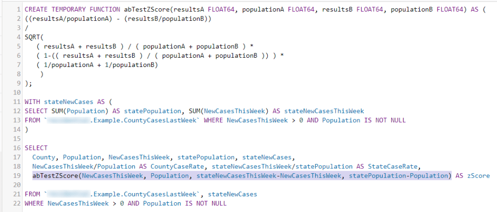
You can copy the abTestZscore function as text from the end of this post.

The function calculates a z-score instead of a p value. There’s a table in the back of most statistics books with a conversion, but you probably only need to know a couple of critical values. A z-score of 2.6 = 99%, 2.0 = 95%. If the z-score is 3, you’re safe in assuming that there is a non-random difference between the two ratios – less than a 1% chance of it being caused by noise in the data. Z-scores can wind up negative as well as positive, but the interpretation is the same.

Note how the abTestZScore function is called. We’re comparing a county’s cases to the rest of the state not including that county – so we remove the county cases and population from the state totals. Z-scores are generated from independent populations.

Here’s a DataStudio presentation of a few results. By the way, the statewide new case rate was 260 (per 100,000 people) that week.

This table lists the counties with the most unexpectedly high number of new cases over the past week. It’s sorted by the Z-score and since all of the values are well over 2.6 we can be very sure that a random fluctation in the number of cases can be ruled out as a cause of the case rate.

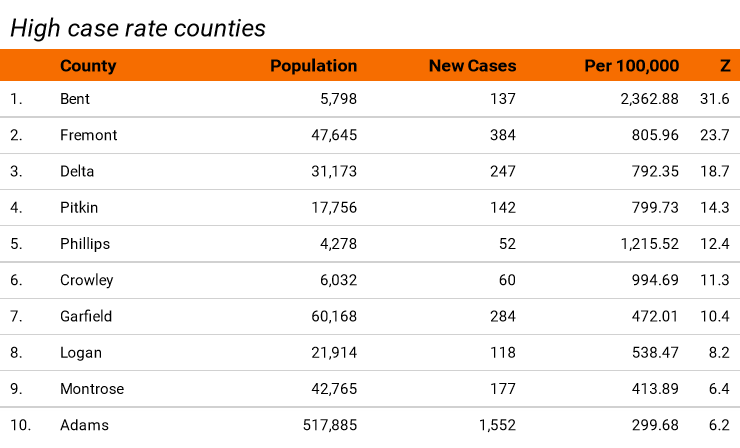
The z-score tells us the most unusual case rates across the state. Since we know that, we can focus limited investigation resources on the top few. By the way, the elevated case rates in the top handful of counties turn out to have been caused by outbreaks in correctional facilities which then spread to the rest of the nearby population from staff members.

Take a look at Adams county at the bottom of the list. For this very large county the difference between the state rate of 260 and the county rate of 300 can’t be explained by random chance. Another explanation needs to be found.

Case rate is the simple proportional comparison. Z-score gives us additional information about whether or not random fluctuation might be involved.

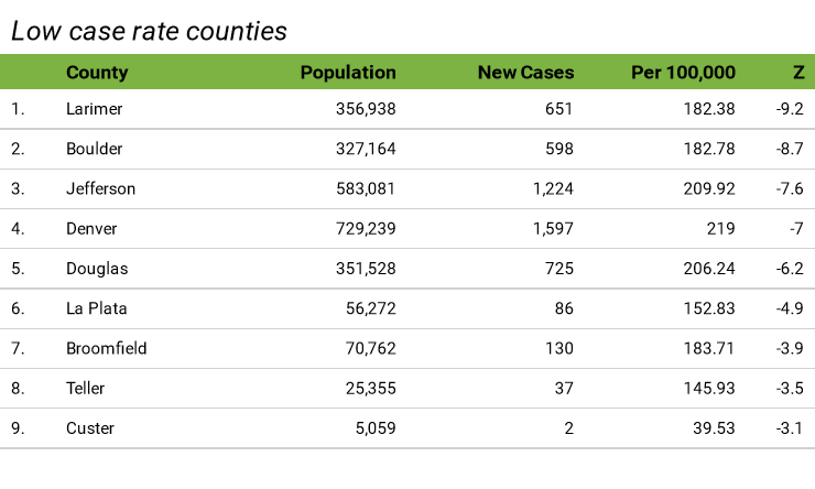
The negative z-scores identify the counties with lower case rates than should be expected from random chance. The first five are among the most-populated Colorado counties. For most of 2020, the big counties had higher case rates than the lower-population counties. Now something is different in these five. Perhaps it’s effective mitigation policies – this data can’t explain it but it gives us a starting point on where to look.

What about that marketing AB test?

Remember that the marketing team ran an AB test to 40,000 people with 15 responses from 1,000 people and 395 from 39,000? Should they be excited that the response rate was 50% higher for the smaller group?

Crunch through the function and you’ll get a Z-score of 1.5 which gives a confidence of less than 90% that the results were anything but chance. If they’d run that test with a split of 2,000 and 38,000 with the same proportion the z-score of 2.2 would give 95% confidence that the test had better results.

By the way, try to agree to a confidence number with your customer before you calculate the scores. That will reduce the desire for them to claim success by backing into a confidence number.

Summary

A little bit of simple statistics can go a long way to improving data interpretation for AB test results. Although a z-score won’t tell you why something happened, it can help you determine how likely it is that chance played a role and to pick out results where further investigation can be productive.

Cut-and-paste AB test function

/*
Function abTestZScore compares results from different sized groups for an AB test
Group A with resultsA (count) and populationA (count)
Group B with resultsB (count) and populationB (count)Null hypothesis is that GroupA and GroupB result proportions are the same. The two groups should not overlap - GroupA and GroupB should not have any of the same members.
Calculate standard deviation (z-score)

Z-score can be positive or negative. Interpret using the absolute value

Zscore Interpretation
2.0 95% chance that results are different
2.6 99% chance that results are different
*/

CREATE FUNCTION abTestZScore(resultsA FLOAT64, populationA FLOAT64, resultsB FLOAT64, populationB FLOAT64) AS (
((resultsA/populationA) – (resultsB/populationB))
/
SQRT(
( resultsA + resultsB ) / ( populationA + populationB ) *
( 1-(( resultsA + resultsB ) / ( populationA + populationB )) ) *
( 1/populationA + 1/populationB)
)
);

Get new content delivered directly to your email. Unsubscribe anytime. I don’t share your email address with anyone.